We will not run this script during the webinar due to time constraints. Instead, the script and all required information are provided below. Preprocessed (i.e., regridded) OISST outputs are available in __data/oisst_processed.
We need to download observed data of sea-surface temperature for our next step of bias correction, which is explained further in the next chapter.
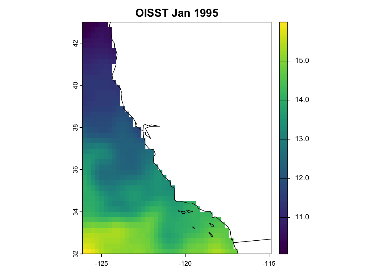
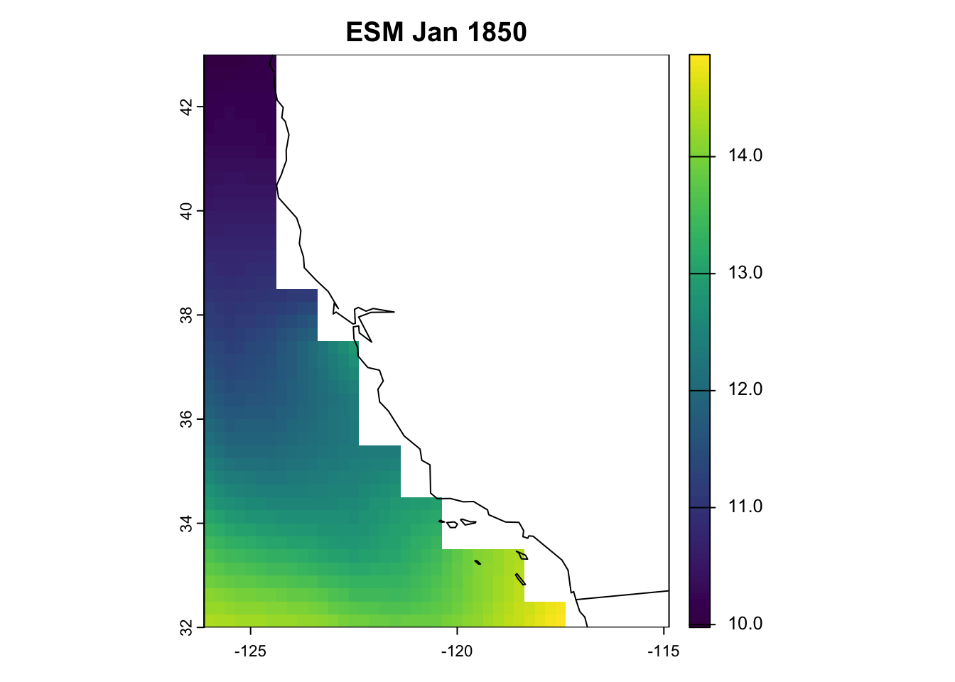
Today, we will use the OISST V2.1 dataset to bias correct our ESM outputs of sea-surface temperature.
The NOAA 1/4° Daily Optimum Interpolation Sea Surface Temperature (OISST) is a long term Climate Data Record that incorporates observations from different platforms (satellites, ships, buoys and Argo floats) into a regular global grid. The dataset is interpolated to fill gaps on the grid and create a spatially complete map of sea surface temperature. Satellite and ship observations are referenced to buoys to compensate for platform differences and sensor biases.
Oceanography terminology: ‘observations’
Whether data are referred to as observations depends on who you to talk to. For the purposes of our workshop, and as marine ecologists, we refer to OISST as our ‘observed’ data set, because it represents ‘real-life’ SST. However, sea-going physical oceanographers might not refer to OISST as observations, because the product represents a series of observations obtained from different platforms (i.e., ARGO, moorings, satellites, ship-borne sensors etc.) that have been ‘modeled’ or ‘interpolated’ into a gridded, cloud-free product. Technically, OISST represents a modeled product based on observations. Rather, they would refer to observations as the raw, unprocessed data coming from sensors themselves. Just something to keep in mind when talking to people from different disciplines.
4.1 Download OISST
Here we define a function that takes two arguments, which denote the start and end of the time period we will use to define our baseline climatology. First, we will download twenty years worth of OISST data, spanning 1995 to 2014, which are our observations. We’ll get into why we chose this time period in the next Chapter. The function downloads daily files of OISST from the index site here.
Code
# Set destination folderoFold <-paste0(pth, "/__data/oisst_raw/")# Set base URLurl <-"https://www.ncei.noaa.gov/data/sea-surface-temperature-optimum-interpolation/v2.1/access/avhrr"# Get the links that appear there as yyyymm datespg <-read_html(url) # Read the HTMLsFld <-html_attr(html_nodes(pg, "a"), "href") %>%# Extract the linksgrep("\\d\\d\\d\\d\\d\\d", ., value =TRUE) # Just the folders with 6 digits (i.e., one per month)# Check what files might already be in the folderf <-dir(oFold, pattern =".nc")# Extract identifiers from the file names - works at level of monthncs <-gsub("oisst-avhrr-v02r01.", "", f) %>%gsub("\\d\\d\\.nc", "", .) %>%unique() %>%paste0(., "/")# Exclude files (months) that are already downlaodedsFld <- sFld[!sFld %in% ncs]download_oisst <-function(yrstrt, yrend) {# Subset sFld to only include time period of interest ind1 <-grep(yrstrt, sFld) %>% min ind2 <-grep(yrend, sFld) %>% max sFld <- sFld[ind1:ind2] length(sFld) #downloading 372 files for 30 yrsfor(i in sFld) { urli <-paste0(url, "/", i) pgi <-read_html(urli) # Read the HTML sFldi <-html_attr(html_nodes(pgi, "a"), "href") %>%# Extract the linksgrep(".nc", ., value =TRUE) # Just the netCDFsfor(j in sFldi) {download.file(paste0(urli, "/", j), paste0(oFold, j)) } }}tic(); download_oisst(yrstrt =1995, yrend =2014); toc()
Jessie speed: ~2 hours (for 20 years of data).
4.2 Preprocess OISST
As with the ESMs, we need to preprocess them. However, OISST are provided as daily files, so we need to calculate monthly averages so they are comparable with our projections. We do this using the -mergetime and monmean operators. Then, as with the ESMs, we need to crop and remap the OISST fields to the same resolution and extent and off the California coast.
Code
oisst_mr <-function(yr,infile =paste0(pth, oisst_pth),outfile =paste0(pth, oisst_pth_proc),xmin =-126, xmax =-116, ymin =32, ymax =43,cell_res =0.25) {# Combine all daily files for X year into one file merged_1yr <-paste0("cdo -mergetime ", infile, "/", "oisst-avhrr-v02r01.", yr, "*.nc ", outfile, "/", "oisst-avhrr-merged_", yr, ".nc")system(merged_1yr) # takes a few seconds# Calculate monthly means for X year mthmeans <-paste0("cdo -L monmean ", outfile, "/oisst-avhrr-merged_", yr, ".nc ", outfile, "/mean_", yr, ".nc")system(mthmeans)# Select SST, crop and remap oisst_regrid <-paste0("cdo -L -select,name=,sst ", "-sellonlatbox,", xmin, ",", xmax, ",", ymin, ",", ymax, " -remapbil,r", 360*(1/cell_res), "x", 180*(1/cell_res), " ", outfile, "/mean_", yr, ".nc", " ", outfile, "/mean_remap_", yr, ".nc")system(oisst_regrid)# Remove temporary files system(paste0("rm ", outfile, "/", "oisst-avhrr-merged_", yr, ".nc"))system(paste0("rm ", outfile, "/mean_", yr, ".nc"))}# Vector of years to processyears <-1995:2014# Modify as neededplan(multisession, workers =14) # Change workers to suit your machinetic(); future_map(years, ~oisst_mr(.x)); toc()plan(sequential) # Return to sequential processing
Jessie speed: ~1-2 min
Once done, we will have a directory containing 20 years’ worth of preprocessed OISST monthly fields.
Here, we’ve created monthly means of OISST from the daily SST fields, to match the temporal resolution of our monthly ESM projections. However, if working with with daily data, you might want to remove February 29th to get around any calendar issues when merging files for bias correction (particularly if working with daily ESM data). This code removes the 29th day of February, and sets the calendar to Gregorian (i.e., 365 days) for infile. We skipped this today to save time, as it can take a while to process (merging 20 years’ worth of daily files is processor-intensive, and results in a large file).