2 Download ESM output from ESGF

2.1 Downloading CMIP6 Earth System Models

The Earth System Grid Federation (ESGF) manages the database for handling climate science data, and supports the Coupled Model Intercomparison Project, which is currently in its sixth iteration (CMIP6).

Today, we will be downloading our model outputs via the ESGF website. We will download the simulations for two models, with the following components:

Component Name	Variable Name	Description
Activity ID	`ScenarioMIP`	ScenarioMIP
Source ID	`ACCESS-CM2`, `IPSL-CM6A-LR`	Model names
Experiment ID	`SSP2-4.5`, `SSP5-8.5` `historical`	Climate scenario (`historical` ranges 1850-2014; `SSPs` range 2015-2100).
Model variant label	`r1i1p1f1`	Model variant indicating the realization, initilization method, physics processes, and forcing datasets used in the model simulations.
Frequency	`mon`	Monthly time-step
Variable	`tos`	Sea-surface temperature

For more information on what ESM components mean, see Table 1 in (Schoeman et al. 2023).

2.2 Download `wget` shell scripts

2.2.1 Navigate to the Metagrid node

Through the website:

Click here to open the website
Click the nodes link to explore the different nodes available (i.e., different data servers)
Click a Metagrid node (i.e., today, we’ll use ORNL metagrid)

You are now on the main website to download CMIP6 output. Ensure CMIP6 is selected under the ‘Project’ heading on the top left, and filter by ‘Only Globus Transferable’. On the left, there are several filters to play with.

2.2.2 Filtering ESM components

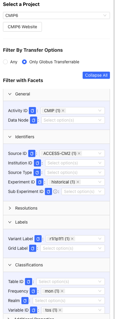
From the left tab, we use the following filters to find the wget script for the ACCESS-CM2 historical simulation:

Click >General, then under Activity ID, click CMIP.
Click >Classifications, then under Variable ID, click tos. Under Frequency, click mon.
Click >Identifiers, then under Source ID, click ACCESS-CM2. Under Experiment ID, click historical.
Click >Labels, then under Variant Label, click r1i1p1f1 (this is the most common variant).

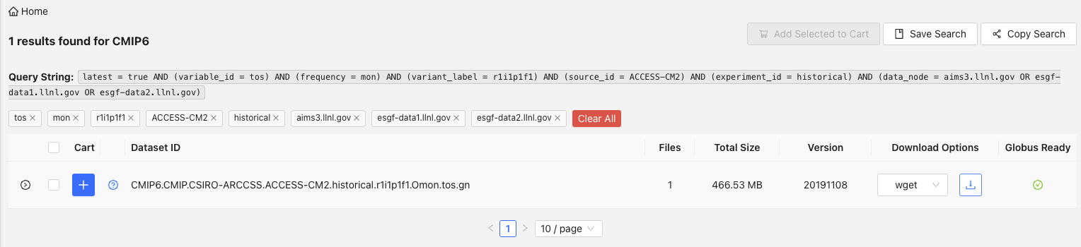
2.2.3 Download `wget` shell script

Then, download the shell script by clicking the Download icon next to the wget download option. This uses wget to download a shell script (i.e., indicated by the .sh file extension) that we will later use to download the file through R whilst interfacing with CDO and the command line.

Once downloaded, move the shell script into the /wget_scripts folder in your project directory.

2.2.4 Rinse and repeat

Now, repeat the process for the SSP2-4.5 and SSP5-8.5 scenarios for ACCESS-CM2, in addition to all three scenarios for IPSL-CM6A-LR. You will only need to change the (i) Activity ID from CMIP to ScenarioMIP, and (ii) Experiment ID filter from historical to ssp245 and ssp585, and You will end up with six shell scripts, three for each model.

2.3 Download `.nc` files with `wget` scripts

Warning: storage

In total, we are about to download eight .nc files that comprise 2.65 GB of data. These are just for two models and two scenarios + historical, at a monthly time-step. Storing ESM outputs can take a lot of space - for example, if you’re working with daily data across multiple models and climate scenarios, you’ll almost certainly need an external hard drive or other storage solution.

We will use wget to download our files from the ESGF Metagrid.

2.3.1 Define dependencies

First, we source our packages and set our directories for where our (i) wget scripts are stored, and (ii) where we will store the ESM outputs.

source(paste0(getwd(), "/__scripts/helpers.R"))

2.3.2 Prepare for parallel processing

We are harnessing the power of parallel processing to download our ESM outputs. We use availableCores() from the parallelly package to tell us how many available cores we have on our machine. I recommend to use whatever the output is minus two, so that your operating system and other background processes can continue working normally. I have 16 cores on my machine, so I’ll use 14 workers.

parallelly::availableCores() # Output says I have 16 cores on my machine
w <- 14  # Leave two cores for other background processes

2.3.3 Function to download files

Now, we write a function that uses the system() function to invoke the terminal from within R to run the wget script, which downloads the ESM file. First, we set our working directory to the full path where data will be stored, which we defined above as /data. Then, we run the system() function to run the wget script using bash via the terminal. Once the script has run and the file has downloaded, we set the working directory back to the root directory.

wget_files <- function(script) {
  setwd(paste0(pth, cmip_pth)) #set directory to where data will be stored
  system(paste0("bash ", script, " -s")) #run wget on the shell script 
  setwd(pth) #set directory back to home directory 
}

Here, we list all wget scripts that we downloaded from ESGF.

files <- list.files(paste0(pth, wget_pth), #full path where wget scripts are stored
                    pattern = "wget", #only files with wget in the name
                    full.names = TRUE #list the full path 
                    ) 
files

[1] "/Users/admin/Documents/GitHub/esmrworkshop_rladies26/__scripts/wget_scripts/wget_script_2026-2-4_12-13-19.sh"
[2] "/Users/admin/Documents/GitHub/esmrworkshop_rladies26/__scripts/wget_scripts/wget_script_2026-2-4_12-14-23.sh"
[3] "/Users/admin/Documents/GitHub/esmrworkshop_rladies26/__scripts/wget_scripts/wget_script_2026-2-4_12-16-43.sh"
[4] "/Users/admin/Documents/GitHub/esmrworkshop_rladies26/__scripts/wget_scripts/wget_script_2026-2-4_12-16-6.sh" 
[5] "/Users/admin/Documents/GitHub/esmrworkshop_rladies26/__scripts/wget_scripts/wget_script_2026-2-4_12-17-4.sh" 
[6] "/Users/admin/Documents/GitHub/esmrworkshop_rladies26/__scripts/wget_scripts/wget_script_2026-2-4_12-5-32.sh"

2.3.4 Run function in parallel

Now, we change to multi-session processing, where multiple workers (sessions) are used to download the files concurrently. We then run the wget_files() function with future_walk() , and use the tictoc package to time how long this takes. Once all files have downloaded, we change back to single-threaded processing.

plan(multisession, workers = w) # Change to multi-threaded processing
tic(); future_walk(files, wget_files); toc() #Run the function in parallel
plan(sequential) # Return to single threaded processing (i.e., sequential/normal)

Jessie speed: 30s to 1 min

Download speeds

Download speeds depend on your Wifi connection, the capabilities of your local machine, and the performance of the server/node you’re attempting to connect to. You can check whether ESGF servers are online here.

We can check the files have downloaded by…

list.files(paste0(pth, cmip_pth))

[1] "tos_Omon_ACCESS-CM2_historical_r1i1p1f1_gn_185001-201412.nc"  
[2] "tos_Omon_ACCESS-CM2_ssp245_r1i1p1f1_gn_201501-210012.nc"      
[3] "tos_Omon_ACCESS-CM2_ssp585_r1i1p1f1_gn_201501-210012.nc"      
[4] "tos_Omon_IPSL-CM6A-LR_historical_r1i1p1f1_gn_185001-201412.nc"
[5] "tos_Omon_IPSL-CM6A-LR_ssp245_r1i1p1f1_gn_201501-210012.nc"    
[6] "tos_Omon_IPSL-CM6A-LR_ssp585_r1i1p1f1_gn_201501-210012.nc"

Great! We have successfully downloaded our ESM outputs.

If your scripts have downloaded data for 2100-2300 (i.e., some models will do this), we can remove those files with the rm argument in shell:

system(paste0("rm ", pth, cmip_pth, "/", 
              "tos_Omon_ACCESS-CM2_ssp585_r1i1p1f1_gn_210101-230012.nc"))
system(paste0("rm ", pth, cmip_pth, "/", 
              "tos_Omon_IPSL-CM6A-LR_ssp585_r1i1p1f1_gn_210101-230012.nc"))

Beware of rm

rm is a handy function for removing files, but there is no way of retrieving them if you’ve accidentally removed the wrong file. So, use this function wisely and make sure you’re 100% confident you’re removing the correct file!