Here are a list of common datasets our team members use/have used in the past, with associated metadata. Check the shared Github repo for R scripts to automatically download data via a thredds server.
Note
Downloading years’ worth of high-resolution ocean data can take some time. Instead of using your home wifi, or even UniSC’s wifi network, we suggest to come in to campus and connect to the uni’s internet with a ethernet/LAN cable (it’s a LOT faster than the wifi!). You can leave your computer somewhere secure overnight to download data automatically via a for loop or with purrr. If you don’t have your own HDR desk, you can leave your laptop running overnight in Kylie or Dave’s office (or on another lab member’s HDR desk, if they’re OK with it), provided they’re in the next day.
Repositories of ocean data
The IMOS Australian Ocean Data Network (AODN) Portal provides access to all available Australian marine and climate science data. Datasets include observations from satellites, moorings and buoys, radars, vessels, Argo floats, animal tracking (satellite and acoustic) and ships. See here for more info on Australia’s national ocean observing system.
Data can also be obtained from NOAA ERDAPP, Copernicus Marine Service, NASA PODAAC etc, but suggest to look at the list on this page first before exploring these data servers/repositories.
Downloading ocean data
There are multiple ways to obtain ocean data. Perhaps the most common method that we use to automate the retrieval of ocean datasets is with a for loop in R, which automatically downloads the files we want from a thredds server.
A thredds (Thematic Real-time Environmental Distributed Data Services) server is a web server that provides metadata and data access for a range of scientific datasets, using a variety of remote data access protocols (such as HTTP and OpeNDAP).
For example, If we want to obtain sea-surface temperature data from IMOS’s L3S 1 day/night multi-sensor product, we can either:
Find the product ourselves on the AODN. Filter the datasets to what we want, as in the below image and select it. Then, click on Info and under Supplementary Resources, click NetCDF files via THREDDS catalog. This takes you to the THREDDS server where you can manually download each file that you want.
Find the product manually on the the IMOS Thredds Server. The file path in this instance, would be /IMOS/SRS/SST/ghrsst/L3SM-1d/dn, which gets us to the same location as the bullet point above.
Write a function in R (recommended) to automatically download the years that we want, direct from the thredds server. You can write a function with a for loop or with the purrr package. Below is a custom function that uses a for loop.
Show the code (for loop)
# Download IMOS SST product# IMOS-SRS-SST-L3S-Multi Sensor-1 day- day and night time- Australia# Metadata: https://catalogue-imos.aodn.org.au/geonetwork/srv/api/records/d7f3178d-869a-4eac-959d-71d1f5e24888# Thredds - https://thredds.aodn.org.au/thredds/catalog/IMOS/SRS/SST/ghrsst/L3SM-1d/dn/catalog.html# Written by Jessie Bolin December 2023 # NOTE: This code will not work if the URL to the THREDDS server changes. If this code# fails, check the URL in the first instance. # Dependencies ------------------------------------------------------------library(XML)library(beepr)library(RCurl)library(lubridate)# Function ----------------------------------------------------------------getIMOSsst <-function(yrst, #start year yrend, #end yeardir ="/Users/jessicabolin/tmp") { #directory yrs <- yrst:yrend #list of years files <-list.files(dir) #list of files already in directory (if any) alldates <-substr(files, 1,8) #dates of files already downloaded (if any)for(i in yrs) { #for each year#sequence of dates from 1st Jan to 31st Dec ds <-seq(as.Date(paste0(i, "-01-01")), as.Date(paste0(i, "-12-31")), by =1) ds <-gsub("-", "", ds) #remove hyphens no <- alldates[which(alldates %in% ds)] #which files are already downloaded? (if any) getnc <- ds[which(ds %in% alldates ==FALSE)] # Which days in year i are NOT already downloaded? getnc <- getnc[!getnc %in% no] #avoid downloading files already downloadedif(length(getnc) >0) { # If there are files that need to be downloadedfor(j in1:length(getnc)) { #for each file# Obtain the URL from the thredds server for each daily file of interest x =sprintf('https://thredds.aodn.org.au/thredds/fileServer/IMOS/SRS/SST/ghrsst/L3SM-1d/dn/%4i/', i) xx = getnc[j] #the date of interest (without hyphens) y ="092000-ABOM-L3S_GHRSST-SSTfnd-MultiSensor-1d_dn.nc"#rest of file name - standard across all files url <-paste0(x, xx,y) #paste them together for the complete URL if (!file.exists(paste0(dir, "/", xx, y))) { #if file exists in our directory, skip itif(url.exists(url)) { # Catch #404 errors download.file(paste0(x,xx,y), #if it doesn't exist, download filepaste0(dir, "/", xx, y),quiet =FALSE) #print progress in R console } #404 if then bracket } #file.exists if bracket } #for loop file bracket } #if bracket } #for loop year bracketbeep(3) #when complete, play a sound} # function bracket# Run function -------------------------------------------------------------options(timeout =1000000) #increase time to 1000000 seconds so downloads will not stop prematurely. Only need to run this once per R session.getIMOSsst(2021, 2022) # Run the function for whatever years you want.
Satellite remote sensing
Tip
The NOAA Coastwatch Satellite Course is an excellent resource for an overview of remote sensing basics, and R tutorials on using satellite data of SST, ocean colour, altimetry etc.
SST
An overview
The ocean and most other objects emit radiation in the infrared and the microwave wavelengths, which can be measured with satellites. Infrared radiation of the ocean comes from the top 10-20 microns of the surface, and are measured by infrared instruments. Microwave radiation results from the topmost 1-millimeter layer, and are measured by microwave radiometers. SST is passively measured using radiometry, meaning the satellite does not ‘emit’ a signal - rather, it just receives a solar radiation reflection. Infrared satellite sensors have better spatial resolution but are more susceptible to cloud contamination than microwave.
The IR sensors have higher spatial (1-4km) and temporal (10-15min, onboard geostationary satellites) resolution, and superior radiometric performance. However, IR sensors cannot “see through cloud”, thus typically limiting retrievals to ~20% of the global ocean, whereas microwave sensors may see through clouds (except heavily precipitating) and therefore have higher coverage, but have coarser spatial resolution (~20-50km) and radiometric performance, cannot be used in coastal and marginal ice zone areas, and may be subject to other errors (due to e.g. radio frequency interference, RFI)
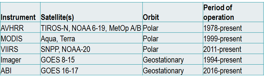
Most of the SST products we use are measured by IR radiometers deployed on a range of polar-orbiting and geostationary satellites.
Raw observations of SST are processed in four different categories. We use either Level 3 or Level 4 processed products. L3 products are composite products obtained by merging all the ocean satellite passages and can be of any spatial resolution. However, some spatial gaps in the data may be present, due to clouds. L4 products are gap-free, where missing data have been interpolated (however, the user does not always know which pixels are ‘pure’ satellite observations, and which pixels are interpolated). Further, when choosing a product, we tend to go for GHRSST products.
Only uses AVHRR on board satellite, and in-situ measurements from ships and buoys
Sea-surface topography
Ocean surface topography is measured using a satellite altimeter. The range from the satellite to the ocean surface is measured using an onboard altimeter that bounces microwave pulses off the ocean surface and measures the time it takes the pulses to return to the spacecraft (a similar concept to echolocation).
Note
In the Bass Strait, you’ll find the IMOS Satellite Altimeter Calibration and Validation Sub-Facility, providing the only southern hemisphere in situ calibration and validation site for satellite altimeters. The facility uses GNSS equipped buoys on the ocean surface as well as an array of sub-surface moored oceanographic instrumentation that includes Current, Wave, Pressure Induced Echo Sounders (CWPIES). Analysis of the absolute bias record over time helps ensure data produced from satellite altimeters are accurate and precise on a global scale.
SSHa, U and V
Sea surface height anomaly (also called GSLA - gridded sea level anomaly). An anomaly is the difference between the long-term average for different regions of the ocean and what is actually observed by satellites in real time. Measuring these differences allows oceanographers and climatologists to detect patterns of global sea level rise, hurricanes, El Niño and La Niña, eddies, boundary currents. When water warms, it expands and raises the surface of the ocean, so measuring the ocean surface height allows scientists to understand how much heat is stored in the oceans. Units are in metres.
U is the east-west component of an ocean current. Positive u means the current is travelling from west to east. Negative u is from east to west. Also called the zonal velocity component.
V is the north-south component of an ocean current. Positive v means the current is travelling from south to north. Negative v is from north to south (like the EAC). Also called the meridional velocity component (think prime meridian).
The AODN provides two datasets that include these three variables. The difference is the time delivery of the products: one is near-real time, and the other is delayed mode.
IMOS OceanCurrent Grided Sea Level Anomaly near real time, thredds
0.2˚
Daily
2011 to present
70E to 170W, 20N to 70S (Australia and surrounds)
Sensors: altimeters on satellites, and tide gauges
Same as above, except data delivered from 1993 to 2020.
Current speed
To get the magnitude (speed) of the current vector, we use Pythagoras Theorem. Units are m/s. This is the square root of the sum of the squares of the u and v velocity components.
\(\sqrt{(u^{2} + v^{2}})\)
Current direction
To get the direction of a current, we turn to trigonometry. We have u and v, and we want an angle. This will require the inverse trig function of tan.
\(\arctan{(v/u)}\)
EKE
Eddy kinetic energy (EKE) is commonly used to study mesoscale eddies. EKE is computed from the zonal (u) and meridional (v) geostrophic velocity components using the equation below. Units are in \(m^2 s^-2\)
\(\frac{u^{2} + v^{2}}{2}\)
Two types exist dependent on the direction an eddy swirls: cyclonic and anticyclonic (note that these reverse if you’re in the northern hemisphere). The centers of cyclonic eddies dimple the ocean surface. In the southern hemisphere, cyclonic eddies are ‘cold-core eddies’, whereas anticylonic are ‘warm-core eddies’.
Keep an ear out for updates on the SWOT satellite mission. SWOT (launched December 2022) will revolutionise our understanding sea-surface topography. SWOT will measure ocean surface topography and land surface water elevation with great accuracy, using interferometry to achieve two-dimensional mapping. Observations from SWOT can be used to better understand ocean currents and processes happening at spatial scales on the order of 15-150 km, something that has not been done before.
Ocean colour
An overview
The Aqua satellite platform carries a MODIS sensor Aqua-MODIS that observes sunlight reflected from within the ocean surface layer at multiple wavelengths. These multi-spectral measurements are used to infer the concentration of chlorophyll-a (Chl-a), most typically due to phytoplankton, present in the water. Aqua-MODIS was launched in 2003. From 1997-2010, chlorophyll-a also came from the SeaWIFS sensor onboard OrbView-2 (SeaStar).
There are multiple retrieval algorithms for estimating Chl-a. Three common ones are the OC3, GSM and OCI algorithms. The OC3 and OCI method is recommended by the NASA Ocean Biology Processing Group. The Garver-Siegel-Maritorena (GSM) method is described in “Chapter 11 of IOCCG Report 5, 2006, (http://ioccg.org/wp-content/uploads/2015/10/ioccg-report-05.pdf).
Note: Most current satellite-based products of ocean colour are affected by cloud contamination, so it’s a good idea to use an 8-day or monthly composite, opposed to a daily product (if that suits your needs).
Chlorophyll-a, Aqua MODIS, NPP, L3SMI, Global, 4km, Science Quality, 2003- present (8 Day Composite) (erdMH1chla8day) files
0.04˚
Global
2003 - present
8-day temporal resolution
Aqua MODIS instrument (visible and IR wavelengths, hence clouds)
SeaWIFS instrument (Orbview-2 satellite (AKA SeaStar)) - OPTICAL WAVELENGTHS only (not IR or microwave, hence clouds)
L3 (has clouds)
FSLE
Backward-in-time FSLEs ridges approximate the so-called Lagrangian Coherent structures. High values of FSLE refer to regions where water parcels that were initially far have converged rapidly.FSLEs are an index of frontal activity.
Maps of Finite Size Lyapunov Exponents and Orientations of the associated eigenvectors (FSLE) (files)
0.04˚
Global
1997 to present
Daily with 8 day delayed time available from 1997. NRT available from May 2018.
Derived from geostrophic currents (DUACS2018 DT MADT UV products)
Note
You will need to create an account with AVISO to access the FSLE products via an FTP client (we recommend FileZilla). More information in the above link.
Bathymetry
The GEBCO_2023 Grid is a continuous, global terrain model for ocean and land with a spatial resolution of 15 arc seconds. It uses as a ‘base’ version 2.5.5 of the SRTM15+ data set between latitudes of 50° South and 60° North. This data set is a fusion of land topography with measured and estimated seafloor topography. The SRTM15+ base grid has been augmented with the gridded bathymetric data sets developed by the four Seabed 2030 Regional Centers to produce the GEBCO_2023 Grid. The Regional Centers have compiled gridded bathymetric data sets, largely based on multibeam data, for their areas of responsibility.
Ocean reanalyses combine ocean models, atmospheric forcing fluxes, and observations using data assimilation to give a four-dimensional description of the ocean (Sorto et al., 2019). Simply put, ocean reanalyses use ocean observations, in conjunction with a numerical ocean model, to create a 3D, gap-free record of the ocean over time. We often use BRAN2020 in our work (developed by CSIRO).
Chamberlain et al. 2021. Next generation of Bluelink ocean reanalysis with multiscale data assimilation: BRAN2020. Earth Syst. Sci. Data, 13, 5663–5688, https://doi.org/10.5194/essd-13-5663-2021
Wedd R et al. (2022). ACCESS-S2: the upgraded Bureau of Meteorology multi-week to seasonal prediction system. Journal of Southern Hemisphere Earth Systems Science 72(3), 218–242. doi:10.1071/ES22026
EAC ROMS (UNSW). Note - this is not operational as of December 2023, and must be requested direct from UNSW’s Coastal and Regional Oceanography Lab). Talk to Kylie if you’re interested in using this.