Intro to netCDF

An overview

Most ocean products come in the format of netCDF. This is the most common data format and file type in the atmosphere and ocean sciences; essentially all output from weather, climate and ocean models is gridded data stored as a series of netCDF files. Satellite data is also often provided in NetCDF format.

The data in a netCDF file is stored in the form of arrays. netCDFs can contain 1D, 2D, 3D or 4D data. For example…

Temperature varying over time at a location is stored as a one-dimensional array. You can think of it as a vector containing elements of the same data type (i.e. temperature values over time at a single longitude and latitude).

An example of a 2-dimensional array is temperature over an area for a given time. Think of an excel spreadsheet, with a table of rows (longitude) and columns (latitude), and each element contains a temperature value for a given time.

Three-dimensional (3D) data is like temperature over an area varying with time. Think of multiple 2D arrays (lat/lon/temp) stacked on top of each other, with each ‘slice’ being a different time period (i.e., day).

- Four-dimensional (4D) data is like temperature over an area varying with time and depth.

Working with .nc files

We use a combination of the ncdf4, terra, raster and stars packages to interact with .nc files in R. If dealing with climate model output, we also often use CDO via the system() function in R or through the terminal/shell.

We also use Panoply (free download) to quickly visualise data from netCDF files before interacting with them in R.

There are many ways to work with netCDFs in R, and a quick google will attest to that. Here are example workflows of using the terra and stars packages to read, manipulate and plot ocean temperature from a .nc file.

With `terra`

#Written by Jessie Bolin (adapted from KScales stars code) December '23.

library(terra)
library(tidyverse)
library(ncdf4)
library(tmap)
library(sf)

### Read the metadata of the file
ncdf4::nc_open("/Users/jessicabolin/Dropbox/ocean_temp_mth_2020_12.nc") -> meta
meta #this shows the dimensions, variables and attributes of the file.

File /Users/jessicabolin/Dropbox/ocean_temp_mth_2020_12.nc (NC_FORMAT_NETCDF4):

     5 variables (excluding dimension variables):
        double average_DT[Time]   (Chunking: [1])  (Compression: shuffle,level 1)
            _FillValue: 1e+20
            cell_methods: Time: mean
            long_name: Length of average period
            missing_value: 1e+20
            units: days
        double Time_bounds[nv,Time]   (Chunking: [2,1])  (Compression: shuffle,level 1)
            _FillValue: 1e+20
            cell_methods: Time: mean
            long_name: Time axis boundaries
            missing_value: 1e+20
            units: days
        double average_T1[Time]   (Chunking: [1])  (Compression: shuffle,level 1)
            cell_methods: Time: mean
            long_name: Start time for average period
            units: days since 1979-01-01 00:00:00
            missing_value: 1e+20
            _FillValue: 1e+20
        double average_T2[Time]   (Chunking: [1])  (Compression: shuffle,level 1)
            cell_methods: Time: mean
            long_name: End time for average period
            units: days since 1979-01-01 00:00:00
            missing_value: 1e+20
            _FillValue: 1e+20
        float temp[xt_ocean,yt_ocean,st_ocean,Time]   (Chunking: [300,300,1,1])  (Compression: shuffle,level 1)
            long_name: Potential temperature
            units: degrees C
            valid_range: -32767
             valid_range: 32767
            missing_value: -32768
            _FillValue: -32768
            packing: 4
            cell_methods: time: mean Time: mean
            time_avg_info: average_T1,average_T2,average_DT
            coordinates: geolon_t geolat_t
            standard_name: sea_water_potential_temperature

     6 dimensions:
        Time  Size:1   *** is unlimited *** 
            long_name: Time
            units: days since 1979-01-01 00:00:00
            cartesian_axis: T
            calendar_type: GREGORIAN
            calendar: GREGORIAN
            bounds: Time_bounds
            cell_methods: Time: mean
        nv  Size:2 
        xt_ocean  Size:3600 
            long_name: tcell longitude
            units: degrees_E
            cartesian_axis: X
            domain_decomposition: 1
             domain_decomposition: 3600
             domain_decomposition: 1
             domain_decomposition: 1800
        yt_ocean  Size:1500 
            long_name: tcell latitude
            units: degrees_N
            cartesian_axis: Y
            domain_decomposition: 1
             domain_decomposition: 1500
             domain_decomposition: 1
             domain_decomposition: 150
        st_ocean  Size:51 
            long_name: tcell zstar depth
            units: meters
            cartesian_axis: Z
            positive: down
            edges: st_edges_ocean
        st_edges_ocean  Size:52 
            long_name: tcell zstar depth edges
            units: meters
            cartesian_axis: Z
            positive: down

    9 global attributes:
        filename: TMP/ocean_temp_2020_12_01.nc.0000
        NumFilesInSet: 20
        grid_type: regular
        grid_tile: N/A
        history: Tue Sep  7 15:29:50 2021: ncap2 -O -s average_DT=average_T2-average_T1 -s Time_bounds(:,0)=average_T1 -s Time_bounds(:,1)=average_T2 ocean_temp_mth_2020_12.nc ocean_temp_mth_2020_12.nc
Mon Sep  6 14:26:43 2021: ncrcat -4 --dfl_lvl 1 --cnk_dmn Time,1 --cnk_dmn xt_ocean,300 --cnk_dmn yt_ocean,300 --cnk_dmn st_ocean,1 ocean_temp_2020_12_01.nc ocean_temp_2020_12_02.nc ocean_temp_2020_12_03.nc ocean_temp_2020_12_04.nc ocean_temp_2020_12_05.nc ocean_temp_2020_12_06.nc ocean_temp_2020_12_07.nc ocean_temp_2020_12_08.nc ocean_temp_2020_12_09.nc ocean_temp_2020_12_10.nc ocean_temp_2020_12_11.nc ocean_temp_2020_12_12.nc ocean_temp_2020_12_13.nc ocean_temp_2020_12_14.nc ocean_temp_2020_12_15.nc ocean_temp_2020_12_16.nc ocean_temp_2020_12_17.nc ocean_temp_2020_12_18.nc ocean_temp_2020_12_19.nc ocean_temp_2020_12_20.nc ocean_temp_2020_12_21.nc ocean_temp_2020_12_22.nc ocean_temp_2020_12_23.nc ocean_temp_2020_12_24.nc ocean_temp_2020_12_25.nc ocean_temp_2020_12_26.nc ocean_temp_2020_12_27.nc ocean_temp_2020_12_28.nc ocean_temp_2020_12_29.nc ocean_temp_2020_12_30.nc ocean_temp_2020_12_31.nc /g/data/gb6/BRAN/BRAN_tmp/daily/ocean_temp_2020_12.nc

        NCO: netCDF Operators version 4.9.2 (Homepage = http://nco.sf.net, Code = http://github.com/nco/nco)
        title: BRAN2020
        catalogue_doi_url: http://dx.doi.org/10.25914/6009627c7af03
        acknowledgement: BRAN is made freely available by CSIRO Bluelink and is supported by the Bluelink Partnership: a collaboration between the Australian Department of Defence, Bureau of Meteorology and CSIRO.

# netCDF files don't often show 'normal' times/dates. Check the units and values of the time slice (note that we already know it should be December 2020)
meta$dim$Time$units #[1] "days since 1979-01-01 00:00:00"
meta$dim$Time$vals #[1] 15325.5
as.Date(meta$dim$Time$vals, origin = "1979-01-01") #[1] "2020-12-16". 
# December 2020! Nice, we have confirmed the time. 

# Read in the data
rast("/Users/jessicabolin/Dropbox/ocean_temp_mth_2020_12.nc") -> w
## print summary of w structure
w
# w has 51 layers, corresponding to depth slices (depth in metres)

class       : SpatRaster 
dimensions  : 1500, 3600, 51  (nrow, ncol, nlyr)
resolution  : 0.1, 0.1  (x, y)
extent      : -9.507305e-10, 360, -75, 75  (xmin, xmax, ymin, ymax)
coord. ref. :  
source      : ocean_temp_mth_2020_12.nc:temp 
varname     : temp (Potential temperature) 
names       : temp_~325.5, temp_~325.5, temp_~325.5, temp_~325.5, temp_~325.5, temp_~325.5, ... 
unit        :   degrees C,   degrees C,   degrees C,   degrees C,   degrees C,   degrees C, ...

names(w) %>% head() #show the names of the first 6 layers
# we can see that each layer corresponds to a different depth slice.
# We already know that there is only one time field, hence why all times are the same

[1] "temp_st_ocean=2.5_Time=15325.5"               "temp_st_ocean=7.5_Time=15325.5"              
[3] "temp_st_ocean=12.5_Time=15325.5"              "temp_st_ocean=17.51539039611816_Time=15325.5"
[5] "temp_st_ocean=22.66702079772949_Time=15325.5" "temp_st_ocean=28.16938018798828_Time=15325.5"

## This is a global field. We may want to crop it to our region of interest.
## filter to crop to region of interest by lon, lat (x, y)
w %>% 
  crop(c(151, 160, -33, -23)) -> x2

## slice to get a depth slice (here, top slice of 2.5m - the surface)
x3 <- x2[[1]]

# set crs
crs(x3) <- crs("epsg:4326") #this is lon/lat WGS84
x3

class       : SpatRaster 
dimensions  : 100, 90, 1  (nrow, ncol, nlyr)
resolution  : 0.1, 0.1  (x, y)
extent      : 151, 160, -33, -23  (xmin, xmax, ymin, ymax)
coord. ref. : lon/lat WGS 84 (EPSG:4326) 
source(s)   : memory
name        : temp_st_ocean=2.5_Time=15325.5 
min value   :                        20.9396 
max value   :                        27.8477

# Plot! the basic way
plot(x3, col = viridis::viridis(255))
maps::map("world", add = T, fill = T, col = "grey")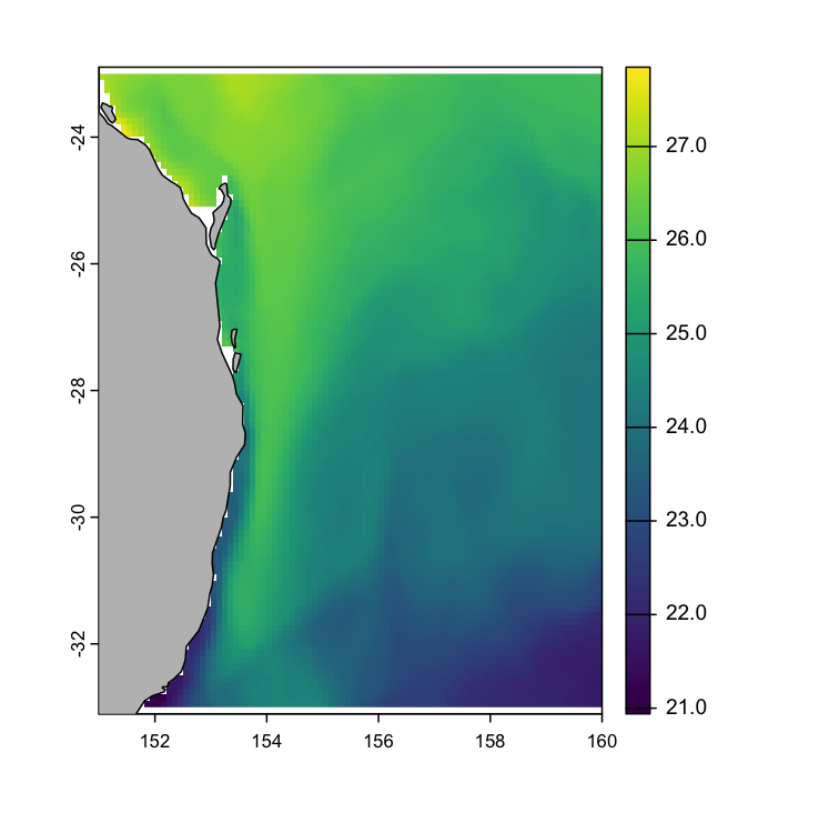

# the fancy way (with tmap)
aus <- rnaturalearth::ne_countries(country = 'Australia', 
                                   scale = 10, 
                                   returnclass = 'sf')

p1 <- tm_shape(x3) +  
tm_raster(title = "SST",
          style = "cont",
          palette = viridis::viridis(255)) + 
  tm_graticules(ticks = T, lwd = 0.5, 
                n.x = 4, n.y = 4,
                labels.size = 1, 
                col = "grey30") +
  tm_legend(position = c("right", "top"),
            legend.text.size = 1,
            frame = T, frame.lwd = 0.001) +
  tm_layout(main.title = "SST for December 2020 (BRAN)",
            legend.title.size = 1.4, 
            bg.color = "white",
            legend.frame = T, 
            fontfamily = "Arial Narrow") +
  tm_shape(aus) +
  tm_polygons()

p1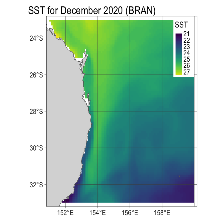

### EXTRACT point values from spatial coordinates (like fishing or animal sightings locations)

## random point (n=50) sample from within the bounding box of x3 (our study area)
pnt <- st_sample(st_as_sfc(st_bbox(x3)), 50) %>% 
  vect() #turn into spatvector so next function will work
pnt

 class       : SpatVector 
 geometry    : points 
 dimensions  : 50, 0  (geometries, attributes)
 extent      : 151.2865, 159.5415, -32.92792, -23.364  (xmin, xmax, ymin, ymax)
 coord. ref. : lon/lat WGS 84 (EPSG:4326)

## extract the values associated with these points
vals <- terra::extract(x3, pnt)
vals %>% head()

  ID temp_st_ocean=2.5_Time=15325.5
1  1                       25.14601
2  2                       25.51429
3  3                       26.54028
4  4                       25.02501
5  5                       23.94579
6  6                             NA

## plot the physical data with point data overlaid. Add to p1, made earlier.
# need to convert the spatvector to a sf object in order to work with tmap.
p2 <- p1 +
  tm_shape(pnt %>% st_as_sf()) + 
  tm_dots()
p2

## we have some NAs as we have sampled over land. Let's remove those and replot.
vals2 <- na.omit(vals)
allvals <- pnt[vals2$ID] #only include the points that are not on land
allvals

 class       : SpatVector 
 geometry    : points 
 dimensions  : 40, 0  (geometries, attributes)
 extent      : 151.6047, 159.5415, -32.92792, -23.364  (xmin, xmax, ymin, ymax)
 coord. ref. : lon/lat WGS 84 (EPSG:4326)

p3 <- p1 +
  tm_shape(allvals %>% st_as_sf()) +
  tm_dots()
p3

## we can convert our extracted temperature values to a data.frame, for visualisation, model fitting, etc.
temps <- as.data.frame(vals2)

# extract associated lat/lons
latlons <- pnt[vals2$ID] %>% 
  st_as_sf() %>% 
  st_coordinates() %>% 
  as.data.frame()

# combine
all_temps <- cbind(temps, latlons) %>% select(-ID)
names(all_temps) <- c("sst", "lon", "lat")
head(all_temps)

       sst      lon       lat
1 25.14601 157.8255 -26.11188
2 25.51429 158.8546 -24.15287
3 26.54028 151.6047 -23.36400
4 25.02501 154.9424 -28.29148
5 23.94579 156.8460 -29.33624
8 24.29825 155.2664 -30.29969

With `stars`

Here is the above code rewritten in stars.

### Reading, plotting and manipulating physical data as NetCDF with package `stars`
### Written by Kylie L. Scales, March 2022
### Comprehensive help for `stars` and mapping to `raster` functions at https://r-spatial.github.io/stars/articles/stars1.html
### Physical data examples from ocean model BRAN2020 (BlueLink Reanalysis), CSIRO. 
### Full info and data download at https://research.csiro.au/bluelink/outputs/data-access

library(stars)
library(cubelyr)
library(dplyr)
library(abind)
library(ggplot2)
library(viridis)
library(ggthemes)

## Download NetCDF from BRAN2020 from NCI data catalogue using THREDDS server
## https://dapds00.nci.org.au/thredds/catalog/gb6/BRAN/BRAN2020/catalog.html
## First, we'll use monthly ocean temperature data for December 2020, from: 
## https://dapds00.nci.org.au/thredds/catalog/gb6/BRAN/BRAN2020/month/catalog.html
## scroll down to file `ocean_temp_mth_2020_12.nc` and click on filename
## click on HTTPServer link for a download of individual file through your browser
## save to your local drive (here, in ~/tmp/BRAN)

## We can automate download of multiple files from NCI, here using one as an example.

### READ the NetCDF file in using function read_ncdf(), and assign to an object, w
read_ncdf("/Users/jessicabolin/Dropbox/My Mac (Jessicas-MBP)/Desktop/Github/ocean_temp_mth_2020_12.nc") -> w
## print summary of w structure
w

## w has one attribute, temperature in °C
## w has four dimensions, xt_ocean (longitude), yt_ocean (latitude), st_ocean (depth), Time
## Time is a POSIXct object with meaningful dates as YYYY-MM-DD. 
## There is only one time value as it's a single monthly field
## There are 51 depth slices, each with a corresponding value (depth in metres)

# select temp and drop singular time dimension ## NB. may need to keep if time matching point data later
x <- w %>% select(temp) %>% adrop()
x

## This is a global field. We may want to crop it to our region of interest.
## filter to crop to region of interest by lon, lat (x, y)
x
x %>% 
  filter(xt_ocean > 140, xt_ocean < 170, yt_ocean > -45, yt_ocean < -5) -> x2
x2

## slice to get a depth slice (here, top slice)
x2 %>% 
  slice(st_ocean,1) -> x3

x3

### PLOTTING using ggplot2()

## single depth layer (top slice)

p1 <- ggplot() +  
  geom_stars(data = x3, alpha = 0.8, downsample = c(1, 1, 1)) +
  scale_fill_viridis() +
  coord_equal() +
  theme_map() +
  theme(legend.position = "bottom") +
  theme(legend.key.width = unit(2, "cm"))

p1

## several depth layers (here, top 12)

x2 %>% 
  slice(st_ocean,1:12) -> x4
x4

## open a new plotting window on a Mac. On a windows machine, use windows() instead
quartz() 

ggplot() +
  geom_stars(data = x4, alpha = 0.8, downsample = c(1, 1, 1)) +
  facet_wrap("st_ocean") +
  scale_fill_viridis() +
  coord_equal() +
  theme_map() +
  theme(legend.position = "bottom") +
  theme(legend.key.width = unit(2, "cm"))


### EXTRACT point values from spatial coordinates (like fishing or animal sightings locations)

## random point sample from within the bounding box of x3 (our study area)
pnt <- st_sample(st_as_sfc(st_bbox(x3)),50)
pnt

## extract the values associated with these point geometries
vals <- st_extract(x3, pnt)
vals

## plot the physical data with point data overlaid. Add to p1, made earlier.
p2 <- p1 +
  geom_sf(data=pnt)
p2

## we have some NAs as we have sampled over land. Let's remove those and replot.
vals2 <- na.omit(vals)
p3 <- p1 +
  geom_sf(data=vals2)
p3

## we can convert our extracted temperature values to a data.frame, for visualisation, model fitting, etc.
temps <- as.data.frame(vals2)
temps

## or, with longitude and latitude as separate columns, rather than point geometries
latlons <- st_coordinates(vals2) # Convert sf point geometries into a matrix of coordinates
latlons <- as.data.frame(latlons) # Convert from matrix to data frame
names(latlons) <- c("lon","lat")
temp2.5m <- as.vector(vals2$temp)
temps <- cbind(latlons, temp2.5m)
head(temps)

An overview

Working with .nc files

With terra

With stars

With `terra`

With `stars`